A simple network traffic model
Hours spent navigating the Perth CBD during my commute has given me too much time to consider what I would do differently; specifically, ``how I would change things to make my commute faster?’’. In reality the challenge of designing a transport network is to build a system that optimises over a diverse population of users: reducing time lost to congestion, being resilient to blockages/incidents, and allowing the city to function efficiently. This already difficult, multi-faceted optimisation is made even more challenging by the presence of unknown (or random) effects such as fluctuating commuter numbers on different routes, the stochastic nature of car accidents (or other road-blocking events), the distribution of driver behaviour and competence, weather events… and many more.
With all of this being said, traffic systems present an enticing modelling challenge that draws on mathematical concepts like networks/graphs and differential equations, an abundance of real-world data, and expert knowledge. In this post I talk through some of early exploratory analysis of some real traffic data.
Problem statement
Main Roads provides a number of real-world data sets such as road geometries, traffic-light locations, and vehicle flux (cars per day) on selected roads. I had three goals for my preliminary analysis:
- ingest the raw data,
- unify/join/relate the different data types and preprocess for downstream analysis, and
- view the datasets on a dashboard for interactive exploration.
As with most problems, I have grand plans for the kind of modelling I could do with this data and the kinds of questions I would like to answer. Some of these questions require sophisticated models for flow on the network, which is too complicated for a ``first look’’ at the problem. As always I find it best to keep it simple to start and to keep my models modular so that simple approximations can one day be substituted by more appropriate ones.
The approach
The data sets are all available from the Data WA, but require processing before they are ready to be visualised on a dashboard. The data sets I used are (i) the Main Roads road network (ii) the Main Roads traffic signal sites, and (iii) the Main Roads traffic digest. The traffic digest represents daily averages of vehicle flux over a six year window.
First, I load the raw data and drop the rows that are outside a predefined box representing the Perth CBD. I also limit to state and local roads. The road network data becomes the basis for my network, with edges represented by road segments and nodes represented by intersections. I merge the traffic digest data onto the road network giving edge weights for a sparse subset of the edges. Finally, I build a second data set of nodes comprising all of the intersections, to which I append an indicator column to flag if that intersection has traffic lights.
The traffic network, intersections (with/without traffic lights), and vehicle flux data are illustrated in Fig. 1, which is a snapshot from my interactive dashboard.
Algorithm details
To estimate traffic on un-monitored road segments I used a graph Laplacian approach. For reasons that I won’t go into, this method is not adequate for my future modelling goals (e.g. intervention studies, congestion analysis, simulation,…), but it allows me to (a) build the rest of the modelling pipeline framework and (b) can still give informative results. In time I will substitute this method for one that better fits my constraints.
First, some terminology. Assume I have a network with $m$ directed edges (road segments) and I have vehicle flow (vehicles per day) on $k$ or these edges, which I denote $y \in \mathbb{R}^k$. I want to estimate the vehicle flux on all of the edges, which I denote $f\in \mathbb{R}^m$. We can build an observation matrix $H \in \mathbb{R}^{k\times m}$ that maps $f$ to $y$ via $H f \in \mathcal{R}^k$, and any deviation between $y$ and $H f$ will be the residual for our model.
The simple, Laplacian smoothing model incorporates two key ideas:
- the difference between $H f$ and $y$ should be small,
- edges that are nearby (adjacent and similar) have similar flows. Expressed mathematically, we model for $f$ as the solution to the optimisation problem given by \(\min_{f>0} \left(||Hf - y||^2_2 + \lambda f^{\rm{T}} L_{\rm{E}}f\right),\) where $\lambda$ is a regularisation parameter (smaller $\lambda$ gives less smooth solutions more closely matching data, larger $\lambda$ gives smoother solutions) and $L_{\rm{E}}$ is the graph Laplacian.
The form of this model plays on a basic trade-off between accuracy (with respect to the observations) and dispersal of information across the graph. It has some nice mathematical properties, including the fact that the optimisation problem is convex (making the optimisation for $f$ a relatively simple least squares problem). The worst thing we could do is get bogged down fitting a overly-complicated model that we plan to replace in the long run!
We can further enhance this model by adding in flux constraints such as “the number of vehicles into a node equals the number of vehicles out plus any sources or sinks”. At this stage I chose not to do this as the available data in its current form isn’t really suitable for such a model, and the diffusion-based model form isn’t one I’ll be using in future analysis anyway.
Findings
Despite the limitations of this simple model, the results are still useful. See Fig. 2 for an illustrative snapshot taken from my dashboard. First, they allowed me to build the pipeline around a dataset with somewhat sensible results, and view these results on a basic dashboard. Second, the broad expected characteristics (such as major artery roads having higher flux) seem to be achieved, allowing for a more informative high level view of traffic in the CBD area compared to the sparse observations.
There’s numerous ways to poke holes in this model, and if you stare at certain parts of the city long enough and you see things that don’t make sense (e.g. parts of East Perth seeing 30 000 cars or more per day, which is a consequence of these segments connecting to the freeway offramp, even though most cars would pass by). My goals for this analysis were very modest though and all I really wanted was to lay the groundwork for future modelling, which I have acheived.
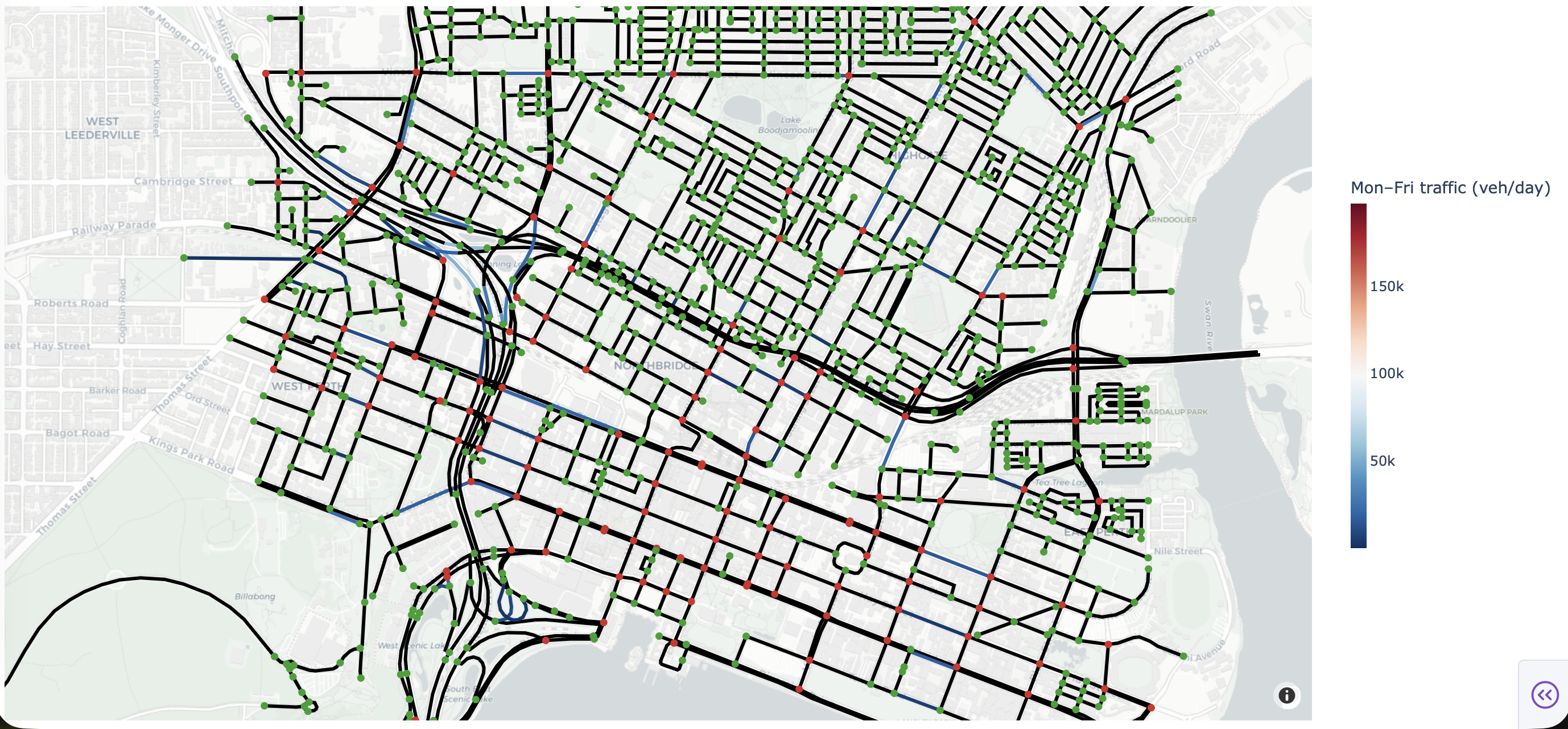
Fig.1 A view of the MainRoads road network data (edges), intersection designations (green points show traffic lights, red points are interesections without lights), and average daily vehicle volume. A black edge indicates no vehicle data for that edge.
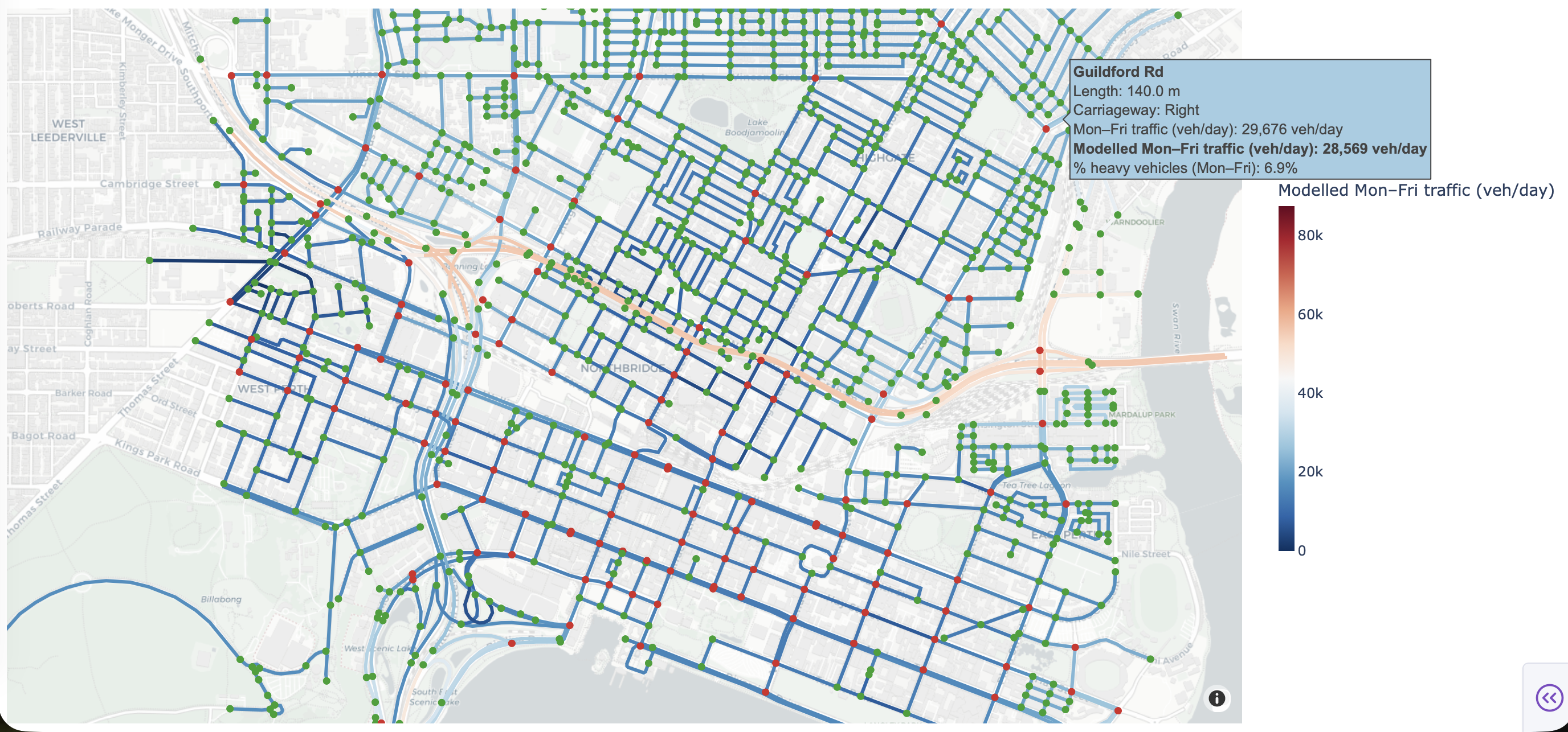
Fig.2 Daily vehicle volume estimated using the graph Laplacian model.