Simulating case data
Simulated or artificial data can serve an invaluable role in building a modelling pipeline. To simulate data we build some assumptions about the data generating process into a model, and use this model to generate artificial observations. Such data can help us to better investigate error structure of our pipeline, test our algorithms, and to better quantify uncertainty. This is because with simulated data we know everything about the data-generating process; we have a ground truth.
A full lesson on errors is outside the scope of this post, but broadly speaking total error can be decomposed into (1) approximation error (model mis-specification), (2) estimation error (finite data), and (3) optimisation error (algorithm).
- If our simulated data comes from a model that closely represents our beliefs about the data-generating process, and this data is fundamentally different to the observations, then this could indicate model mis-specification.
- Because we can generate as much data as needed, we can see how the pipeline performs with different volumes of data, and understand if the available observations are likely to be sufficient.
- Comparing the inferred parameters to the known input parameters allows us to test and fine-tune the performance of our algorithms.
Problem statement
The challenge is simulating case data that is suitable for (i) illustrating the value of the dashboard we built and (ii) for testing our methods. We must encode enough of the data-generating process to be representative of the real-world data, but we don’t want data that is so complicated that we can’t identify where things go wrong if needed.
The primary dynamic that should be incorporated is that of infection: each local case is the result of an infection from a parent, forming a tree-like network originating at each imported case. It’s important that our simulated data has this tree-like structure where local cases are not independent.
For the sake of visualising the data, a second desirable feature of the simulated data is that the infectiousness of the cases depends on the environment, particularly rainfall. I wanted to impose this because the relationship between transmission rate and rainfall was something that we were able to identify in the real-world data when plotted appropriately on our dashboard.
Our approach
My simulation process was as follows:
- Simulate case-importations uniformly in space and time.
- For each case, the reproduction number, Re, is a random variable that determines how many subsequent cases are generated.
- Subsequent infections emerge 7 days after infection at a random distance from the source case, with the probability of distance from the source following a Gaussian distribution around the source (i.e. more likely to occur closer than further away).
- Each transmission chain is followed until either no more cases result (Re=0) or an end date is reached.
To impose environmental dependence, I sampled Re from a Poisson distribution, with λ (mean and variance) being a function of rainfall.
Algorithm details
One challenge of simulating data like this is that we don’t know how many cases we will have until we’ve generated them. So we can’t just write a loop that goes through case-by-case until the simulation is complete. The key data structure that simplifies this process is a queue, where elements are sequentially removed from the start of the queue and new elements are added to the end (first in first out). Thus, for a single imported case we can build a queue by starting with that case, simulating the infections from this case and adding them to the end of the queue, removing the original case from the start of the queue, and then moving on to the next element in the queue and repeating this process. For each imported case we can simulate new infections, adding and removing from our queue, until the queue is empty (the outbreak has subsided) or the end date is reached.
Findings
The best place to view the simulated data as well as some real rainfall data on the dashboard HERE.
Below I illustrate the imported cases (Fig. 1) and an animation illustrating the outbreaks (Figures 2 and 3). For the P.falciparum species of malaria (Fig. 2), Re was rainfall dependent, which it wasn’t for P.vivax (Fig. 3). This gives rise to different spatiotemporal dynamics driven by the underlying rainfall patterns.
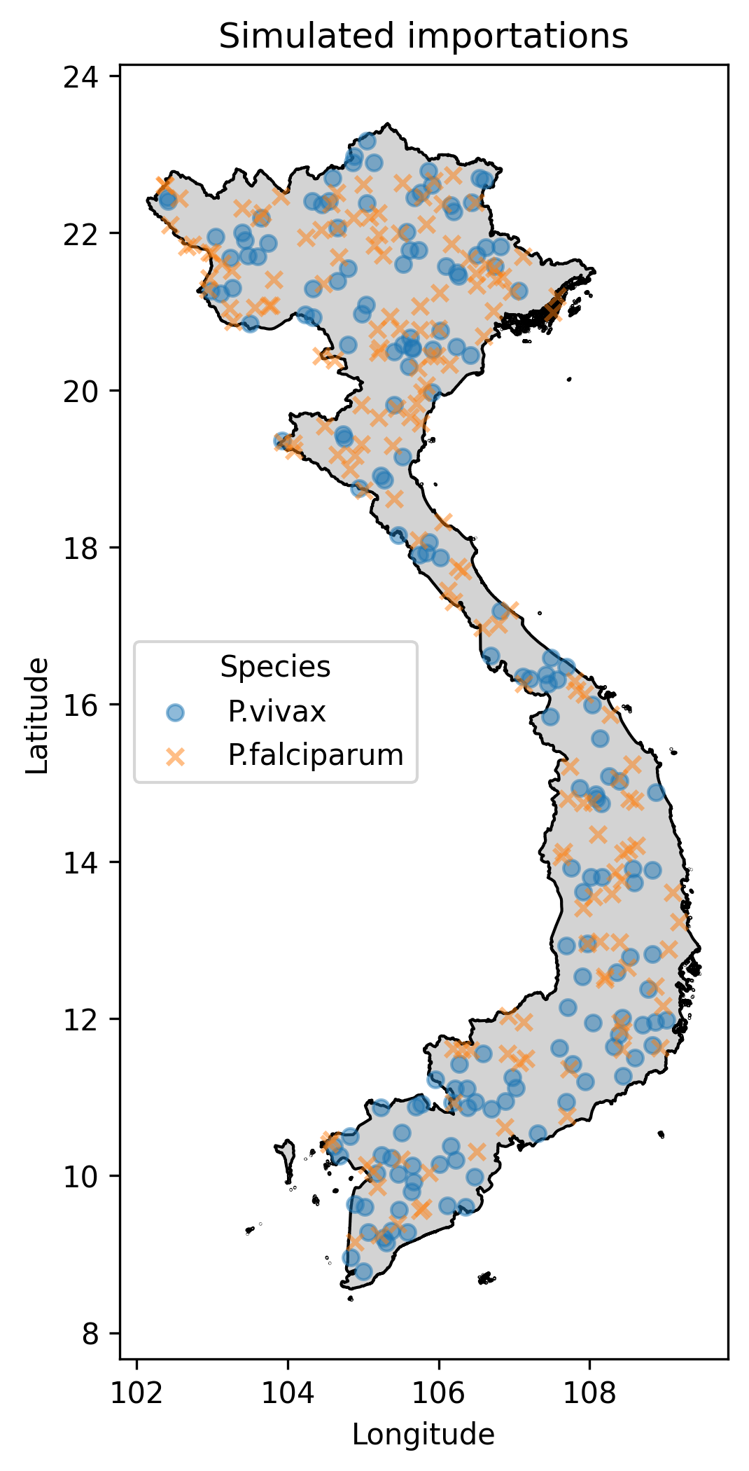
Fig.1 The simulated imported cases, where the marker shape indicates malaria parasite species.

Fig.2 The simulated P.falciparum cases through time, colour-coded according to index case (i.e. which imported case began the outbreak).
Fig.3 The simulated P.vivax cases through time, colour-coded according to index case (i.e. which imported case began the outbreak).