A traffic model with congestion
In my previous post, I outlined some of my early exploration of traffic data and modelling. Before I can begin investigating my network optimisation questions, I need to build in some realistic traffic dynamics. In particular, I want to be able to perturb the network, and look at the system-wide response.
A key dynamic I want to incorporate is road capacity; if too many vehicles attempt to use the same segment, congestion reduces the average speed of vehicles. This means that (i) the most efficient routing between two points does not just send all vehicles along the same edges and (ii) if one path becomes less efficient (or is removed), the redistribution of vehicles to other segments of the network should be aware of the detrimental impact of too many vehicles on each segment.
By simply adding congestion dynamics to the network, I can start to perform a range of scenario analysis. In each scenario—more vehicles on the network, edge removal, edge addition, traffic light optimisation—I can summarise some key quantities: traversal time for different routes on the network, and a secondary quantity time lost to congestion. These two metrics will be key to quantifying the impact of interventions/events, and optimising over the network.
Building a realistic transport network using real data with realistic re-routing dynamics is a challenging enough task that it should be broken into bite-sized tasks. So in this post I will cover some exploratory work to try and understand the relationship between congestion and traversal speed.
Problem statement
To incorporate road capacity and its impact on vehicle speed across the network we need to
- explore the relationship between vehicle volume and vehicle speed
- parameterise this relationship
- train a model for volume vs speed that can be applied to all edges in the network. In this post I only cover point 1, as there is a rich set of traffic dynamics to be observed in the data alone.
The approach
On top of the network data used in Post 1, I downloaded the hourly and quarter hourly data from the Main Roads Data Map. For each observation site we have obverved vehicle flux and binned speed data (in 20km/hr incremements). The vehicle volume measurements are per quarter hour (i.e., cars in 15 minutes).
Findings
Viewing the volume vs speed plots for all of the sites is surprisingly informative. In most places the behaviour is as expected: cars travel near the speed limit when volume is low, and as volume increases the speed drops. See Fig 1a for a typical profile. In some places, the drop in speed is quite dramatic above critical volume thresholds (Fig 1b).
When average speed differs from speed limit
In a number of cases, even when the vehicle volume is low, the average speed is not equal to the speed limit. In fact, it’s surprising how often this occurs (see examples in Fig 2). In some cases (particularly where the low-volume speed is below the speed limit), I suspect the measurement is taken at points where vehicles have yet to get up to speed, such as on-ramps or just after traffic lights. In many cases it’s not clear why vehicles are 15km/hr above or below the speed limit. My intention has always been to use the speed-limit data (modified by congestion) to compute traversal time, but seeing how frequently the vehicle data disagrees with the set speed limits, I may have to reconsider!
Volume vs Speed
I observed three charactersitic curves for volume vs speed:
- Linear slowing (Fig 3a)
- Saturation (Fig 3b)
- Constant speed (Fig 3c) In Case (1), vehicles steadily slow as car volume increases. In Case (2), cars slow linearly with increasing volume until a critical volume at which speed drops drastically (traffic jam!). In Case (3), there’s no apparent slowing with vehicle volume. From a modelling perspective, there probably isn’t three distinc cases, just different regimes. The linear phase could be considered being pre-traffic-jam, but with sufficient car density for interactions; that is, these edges just haven’t been observed above the critical threshold. Furthermore, road segments with Case (3) are so far below capacity that there’s no interaction between vehicles. That is, these supposed three response types are all subsets of observations in different regimes.
Thus, I’ve found that my capacity model could have three parts: a low-interaction component, a linear interaction component, and a traffic-jam (oversaturation) component.
Hysteresis
One observation that warrants further investigation is the hysteresis behaviour that emerges for some segments (see Fig. 4). In these cases, the volume vs speed curve is different in the morning and evening. Why this occurs? I’m not sure yet. It may be that when the roads are clear (in the morning) cars can fly through without interacting, but after the slow-down they must all move at slower speeds. This phenomena may relate to the quadratic flux that emerges using the so-called Greenshields Model (linearly decreasing vehicle speed with vehicle density on the road) when modelling traffic using a hyperbolic, first-order partial differential equation (which I might cover in another post).
Is this important? Probably not too important for the low-stakes analysis I’m doing here, but worth keeping in mind.
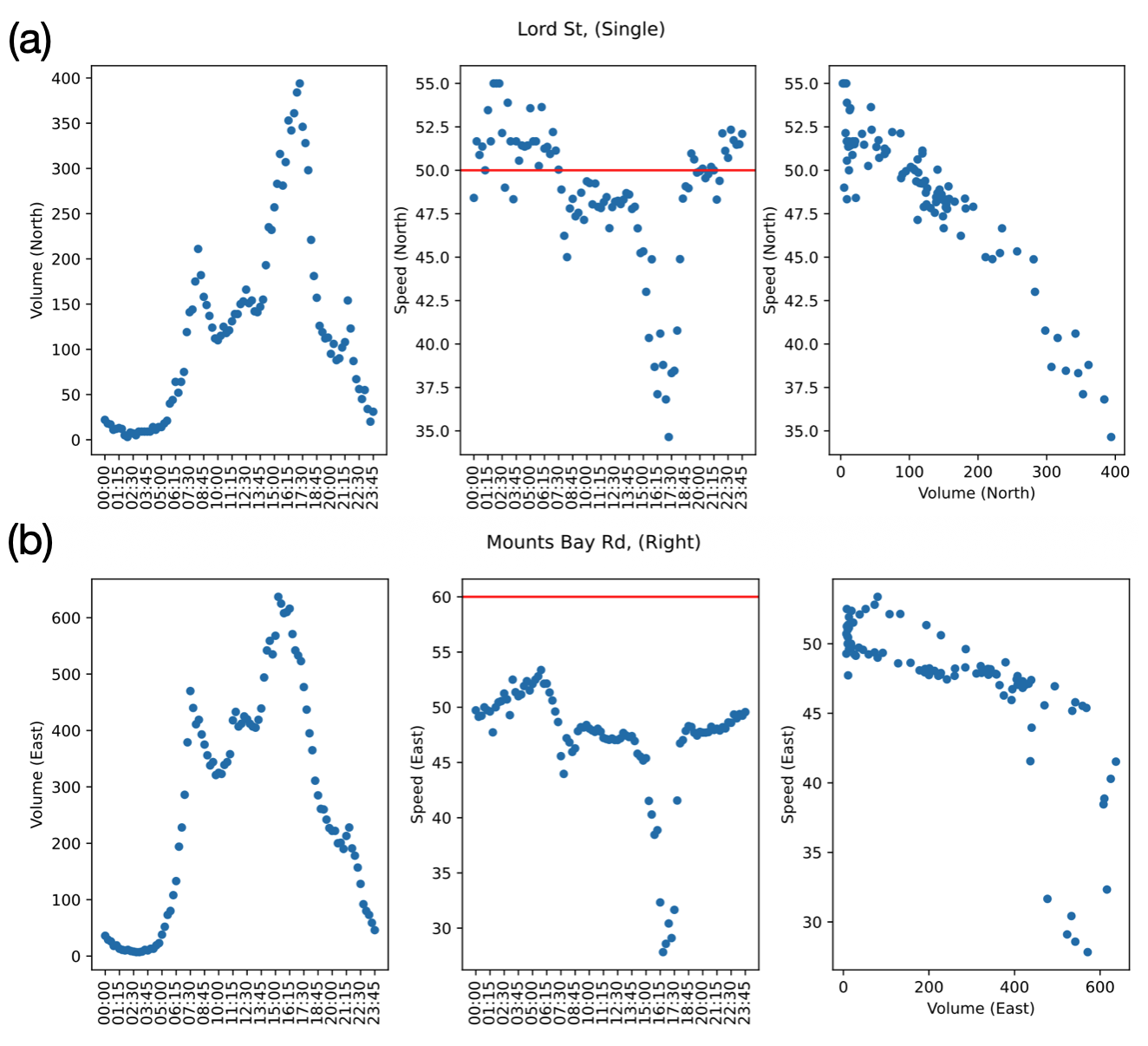
Fig.1 Vehicle volume and speed for (a) Lord Street and (b) Mounts Bay Road (right).
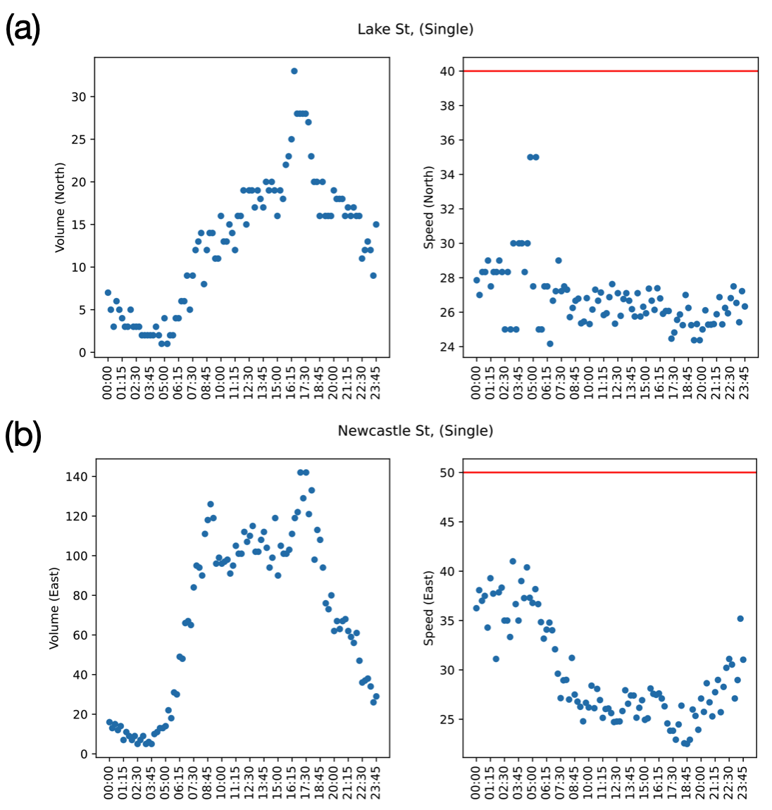
Fig.2 Examples of sites where the observed vehicle speeds differ (even with low vehicle volume) from the speed limit.
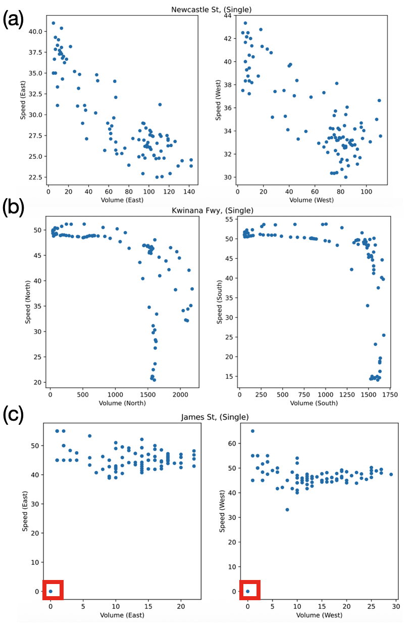
Fig.3 The three characteristic vehicle volume vs speed relationships: (top) linear, (middle) saturation, and (bottom) constant. The red box shows a point with no vehicles, and therefore no speeds, which could be removed for future analyses.
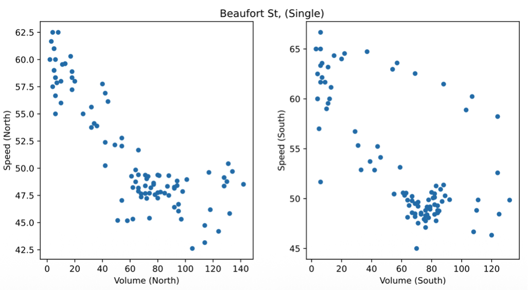
Fig.4 An example of observed hysteresis behaviour. On the same road (Beaufort Street South) two different average vehicle speeds were observed for the same vehicle volumes (depending on the time of day). In this instance, vehicles had higher average speeds (with the same vehicle flux on the roads) in the morning until around 100 vehicles/0.25hr when the morning traffic jam chokes up the roads.