A traffic model with congestion (Pt. 2)
In my previous post, I discussed how congestion must be accounted for in my network-traffic-model so that I don’t get trivial (overly simple) solutions. I also explored some of the data and found that vehicle-vehicle interaction is non-linear in the total number of vehicles using the road segment: at low vehicle volumes speed is independent of vehicle volume, for higher volumes the speed can begin to decrease, and at some point the speed can drop drastically (traffic jam!).
In this post I want to formalise this congestion behaviour. Specifically, I want to estimate a relationship between the time it takes to traverse a road segment and the number of vehicles concurrently using that road segment. We’ll call this traversal-time vs flow, where flow is the number of vehicles on the road segment per hour, and for consistency the traversal-time will be measured in hours. My goal here is not to re-invent the wheel, but to just impart realistic capacity relationships onto my transport network so that I can start to explore the structure of the network. Note that my modelling philosophy is to start simple, but use a sufficiently modular design so that the weaker parts of the model can be substituted for stronger parts later (if needed).
Problem statement
As a reminder from the last post, my goals were as follows:
explore the relationship between vehicle volume and vehicle speed- parameterise this relationship
- train a model for volume vs speed that can be applied to all edges in the network. In this post I will look at point 2. In particular, I’ll introduce a capacity-constrained traversal-time vs flow model, fit this model to the available data, and then discuss some of the findings.
The approach
On top of the network data used in the previous two posts, I added ‘road-segment length’ as a column to my data set, as I need this to comute the traversal time.
I’ve chosen to use the Bureau of Public Roads (BPR) function to represent the travel-time–flow relationship; namely, \(t_{e} = t_{0}\left[1 + \alpha \left(\frac{q}{C_e}\right)^{\beta} \right],\) where $t_{e}$ is the time taken for a vehicle to traverse the edge, $t_0$ is the free-flow time taken (without any traffic), $q$ is the vehicle flow, $C_e$ is the road-segment capacity, and the parameters $\alpha$ and $\beta$ are shape parameters. Conventionally $\alpha=0.15$ and $\beta=4$, but expanded models may fit these parameters to data.
The parameters in this model are easily interpretable. $\alpha$ represents the proportional delay in travel time when the flow is equal to capacity $C_e$. So, $\alpha=0.15$ implies that when $q=C_e$, the time taken to traverse the edge is $15\%$ longer than the free-flow traversal time. The parameter $\beta$ determines how rapidly things grind to a halt when flow exceeds capacity. The larger the value of $\beta$, the faster $t_{e}$ grows with $q$ for $q>C_e$.
Having established the model, the key steps are as follows:
- Compute $t_0$ for each edge with data by dividing the road segment length by the free-flow velocity (inferred from the data for low flows).
- Compute $t_{e}$ for each data point by dividing the velocity by the segment length.
- For each edge fit the BPR function to estiamte $C_e$. In this case I used a least_squares regression with a “soft_L1” loss function (so that outliers don’t sway the fit too much).
Findings
The result of this process is a number of $C_e$ values for select edges in the network. From a quick visual inspection of the outputs—plotting the speed vs flow data, but colouring points where flow is over capacity—I find that the model seems to provide sensible results. What I was hoping to build is a model for edge travel time that slowly grows with increasing flow and then rapidly blows up with flow above a capacity, which this model seems to provide.
The data for East Parade (right) illustrated in Fig. 1 demonstrates this behaviour clearly. For both north and south traffic, when the flow exceeds around 400 cars per hour, the traffic grinds to a halt. In another case, Beaufort Street (Fig. 2), the capacity corresponds with the flows at which the vehicle speed dip below the marked speed limit. In this example the capacity is less of an indicator of jamming behaviour than of a point at which travel time starts taking longer than expected.
The story is not always so clear. Take, for example, Lord Street (Fig. 3), for which there is large volume spikes during peak hour, but only marked jamming in one direction (south). Interestingly, there is still a dip in speed during the evening peak hour (north), but even after the volume starts to decrease, the speed doesn’t immediately return to normal; when traffic has built up, there will be some delay in the return to free-flow conditions.
There is a clear distinction between the capacity of local and state roads, which makes sense given the different nature of these roads (Fig. 4). This distinction will be central to any model that extends these estimated capacities to road segments with no data.
Final thoughts
What We’ve built is a pipeline step that allows us to infer realistic road-segment capacities, and we can now decide how to extend these values to unobserved edges in the network (i.e., edges without data). I will most likely predict static capacities to start, but for robust uncertainty analysis I can also train a probabalistic model for $C_e$ based on the road features and answer future questions using stochastic frameworks.
This analysis shows that even very simple, limited models can still be useful. As long as the behaviour of the system is qualitatively correct, we can still understand the interacting parts and potential feedback loops. This lets us rapidly build a data-driven simulation infrastructure, at each step overcoming the technical/implementation hurdles, without getting too bogged down in quantitative accuracy; that can come later!
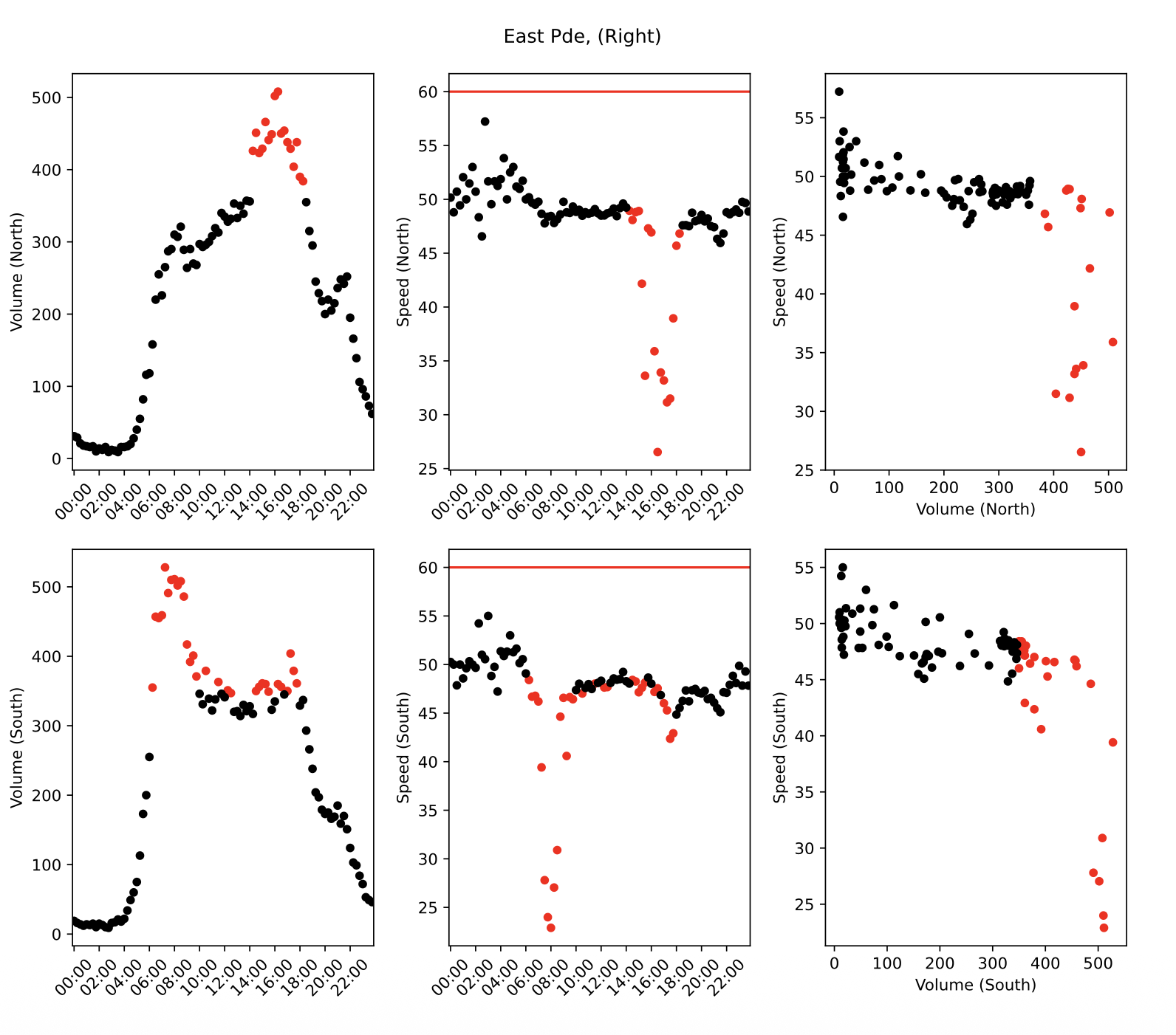
Fig.1 Vehicle volume and speed for East Parade, with times where flow exceeds capacity highlighted in red.
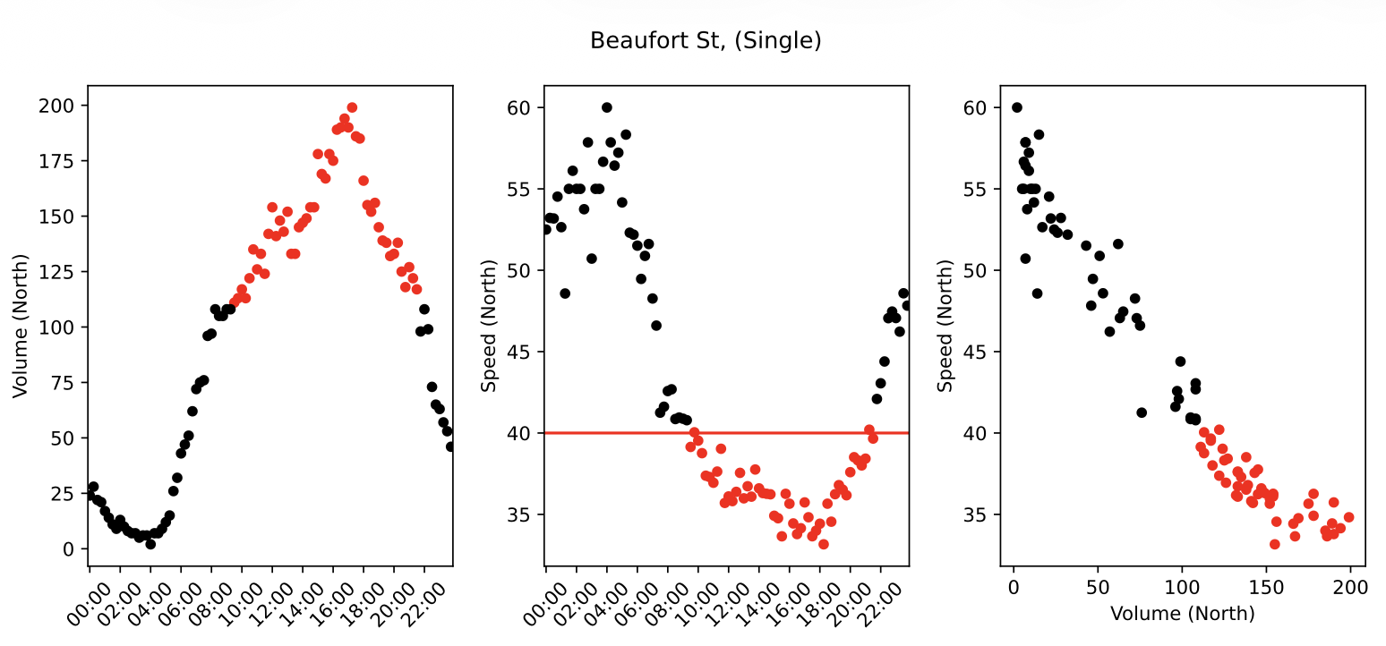
Fig.2 Vehicle volume and speed for Beaufort Street. Flows exceeding capacity are coloured red. The red horizontal line indicates the speed limit.
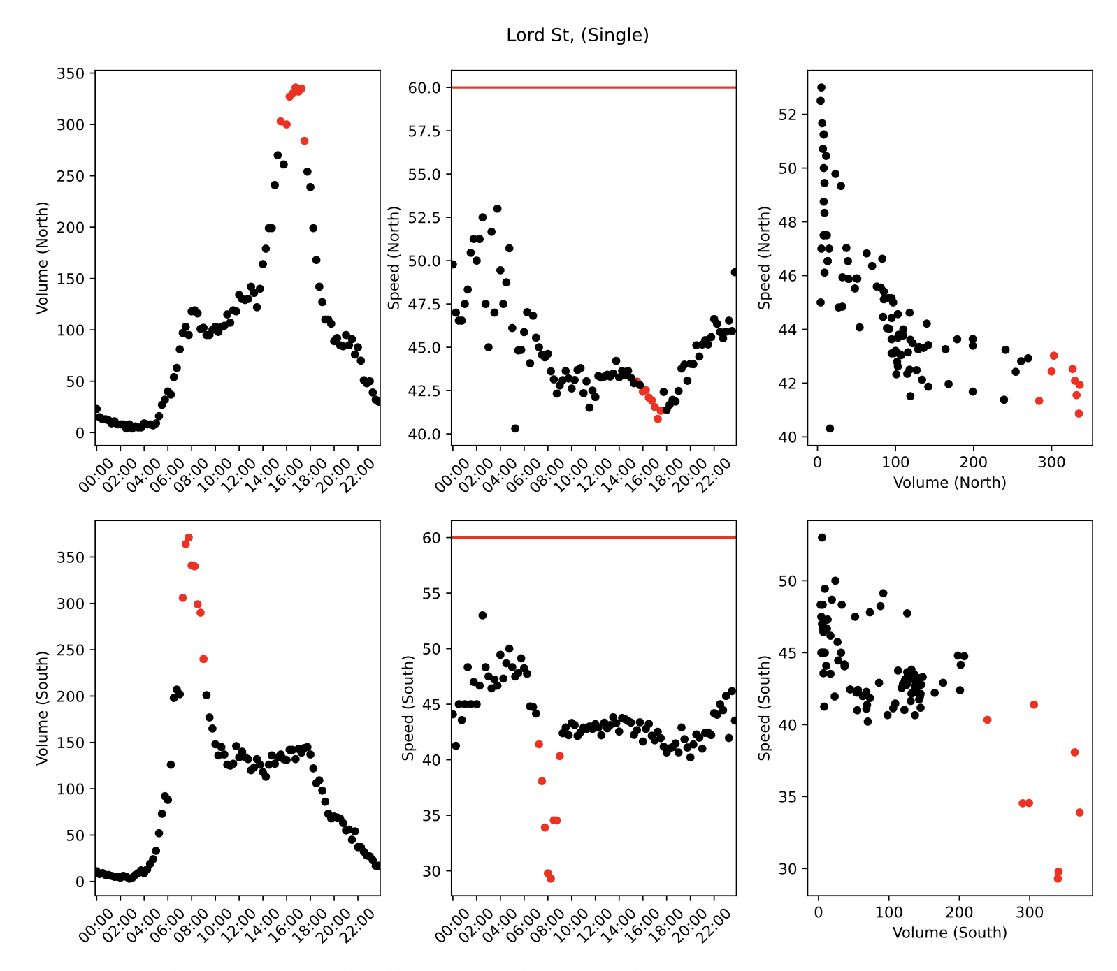
Fig.3 Vehicle volume and speed for Lord Street, indicating a less clear flow vs speed relationship. In this case, particularly for the northbound route, the capacity is less of a ‘critical value’
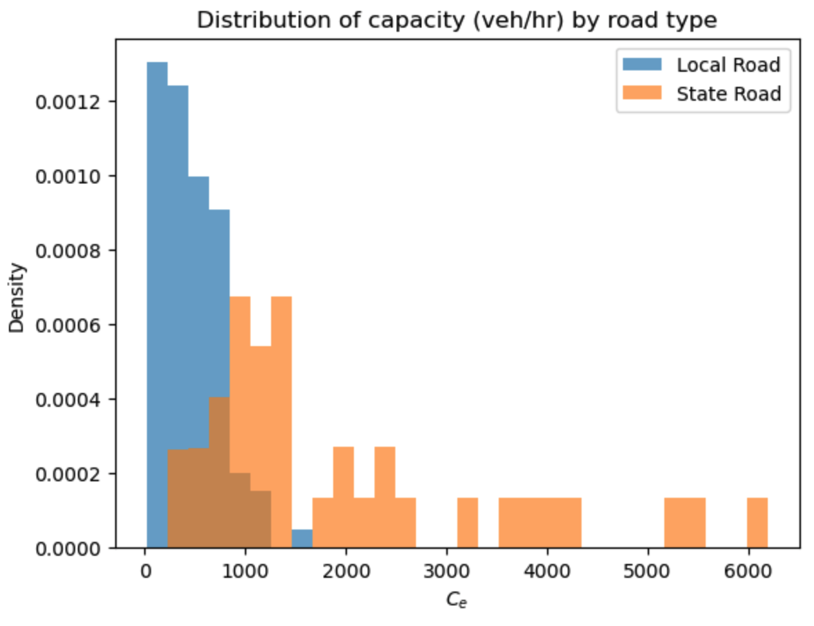
Fig.4 The density of estimated capacities distinguished by road type. The state roads typically have much larger capacities than local roads..