Network flow problems in the city
In my previous post I introduced a congestion model to account for road capacity limits. In the so-called BPR model, vehicle volumes near the capacity of the road-segments results in increased travel times, which sharply increase beyond the capacity. This is a soft capacity that allows for higher volumes, but heavily penalises them. In this post I will treat these capacities as hard limits, and explore a range of network flow problems on this graph.
There are three canonical network flow problems that I’ll look at in this post
- Shortest path,
- Maximum flow,
- Minimum-cost flow. Throughout, I’ll assume that the inferred edge-vehicle-fluxes form a background flow, and the modelled capacities are hard constraints; thus, each edge will have a residual capacity and a volume-dependent traversal time. If the modelled vehicle flux is above capacity, which is more than likely given I’m using peak hour traffic data, then that edge allows no additional volume and is effectively removed from the transport network.
Problem statements
Shortest path
The shortest path problem is to find the path, $P$, of edges between vertices $s$ and $t$ with the smallest total cost (i.e., travel time). The inclusion of an edge in the path comes with a cost (traversal time) $c_e$. So, our objective is to find $P$ such that \(\min_{P:s \rightarrow t} \sum_{e\in P} c_e.\)
Maximum flow
For a given set of origin nodes, $O$, and destination nodes, $D$, the maximum-flow problem is to determine the maximum possible output from the origin nodes that can traverse the network (using only the residual capacity of the edges) to the destination nodes.
The simplest formulation of this problem is for a single fixed source, $s$ and sink, $t$. The flows on the edges, $x_e$, are bounded by the residual capacity, $r_e$. Formulated as an LP, we seek to solve the following optimisation problem \(\max_x \left[\sum_{e\in \delta^+ (s)} x_e - \sum_{e\in \delta^- (s)} x_e \right],\) where $\delta^+$ denote outgoing edges from the source and $\delta^-$ are incoming edges, subject to the residual capacity constraints on all edges $E$, \(0 \leq x_e \leq r_e,\quad \textrm{for} \quad e \in E,\) and the conservation of flow constraints at all vertices (excluding the origin/destination) $V\backslash {s, t }$, \(\sum_{e\in \delta^+ (i)} x_e - \sum_{e\in \delta^- (i)} x_e = 0, \quad \rm{for} \quad i \in V \backslash \{s, t \}.\) To generalise this with more sinks/sources we simply ammend the objective to include the additional sources, and the conservation constraints to further exclude the new sources/sinks.
The minimum-cut theorem allows for a much more efficient routine for computing the optimum value. The theorem states that the maximum flow from source to sink equals the total weight of the edges in a ``minimum cut’’, where a minimum cut is the smallest total weight of edges that, if removed, disconnect the source and sink. The edges comprising the minimum cut are the bottle-neck edges, so it doesn’t matter how much capacity the rest of the network has, these edges limit our flow between source and sink.
Minimum-cost flow
In contrast to the maximum-flow problem, the minimum-cost flow problem is to determine the cheapest (in this case, least total time) routing of the supply from the origins to the destinations. So, with the same constraints as the maximum-flow problem, the new objective is given by \(\min_x \sum_{e \in E} c_e x_e,\) where $c_e$ is the cost (traversal time) of using that edge.
The approach
To solve the shortest path problem, we use Dijkstra’s algorithm from Python’s NetworkX library.
For the maximum-flow problem we use NetworkX’s max-flow and min-cut routines. By exploiting the minimum-cut theorem, we can capitalise on the network structure, and avoid the overhead and more complicated matrix operations required of a Pyomo LP.
For the minimum-cost flow problem we use the Pyomo framework to formulate the problem (decision variables, cost function, and constraints) and either HiGHS or Gurobi as the LP solver. Out of curiosity I implemented both solvers, but for small problems of this nature there is no practical differences in runtime or solution accuracy.
Exploratory dashboard
One option to test these solvers and explore the results is to configure some sample problems and view the solutions. Another, more interactive way, is to adapt the dashboard from my previous post to explore different configurations and solver response. I built a flexible dashboard that allows me to select a number of origin and destination nodes, then solve either the maximum-flow problem or the minimum-cost-flow problem. A snapshot is of the dashboard is illustrated in Fig 1.
Findings
Playing around with the dashboard is incredibly useful. By testing different configurations, I can start to wrap my head around the network structure of the CBD, and new questions spring to mind. For example, what if some of the most commonly active edges were removed (through congestion or road closure etc.)? Which parts of the city are not well serviced? To answer these questions I would devise more structured, targeted approaches. For example, remove individual selected edges from the network and re-compute maximum flows (or min-cost flows), tabulating the change in capacity and visualising the sensitivity of the network to this kind of disruption.
More generally, the purpose of solving these fundamental network optimisation problems is to build on them to ask/answer more sophisticated questions in the future.
Despite the components theoretically accounted for in this transport network—speed limits, capacity constraints, and estimated baseline volumes—it still feels like there’s some ingredients missing; in particular, traffic lights and queueing. At this stage of the process I’m also thinking about whether or not to integrate different sources of traffic data, as the current Main Roads data set is a bit sparse. This means that the congestion/volume models are doing a lot of the heavy lifting in places where real data would be much more valuable.
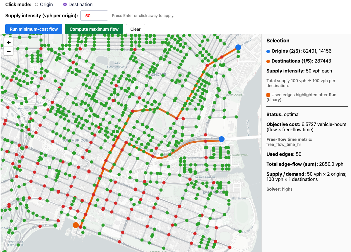
Fig. 1 An example of the dashboard built to explore network optimisation problems. Orange edges are those active in the minimum-cost flow solution. Blue nodes are the two origins, and the orange node is the destination.